Kalman Filters

A lot of my work has, historically, been based around (Ensemble) Kalman filters. On this page I have some resouces which I hope will help you get more to grips with them.

The underlying mathematics can be a little opaque, so I have tried to visualize the process here.

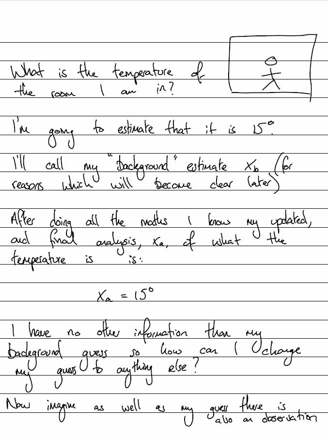
At the 2021 International Union of Radio Science (URSI) I gave a tutorial describing the derivation of the Ensemble Kalman Filter directly from Bayes’ Theorem. Unfortunately the tutorial was not recorded, but my notes are available to anyone who is interested:

However, the best way to learn about Kalman filters, is to play with them. Here is a fun little problem to get you thinking about them.

Imagine dropping a bouncy ball (vertically) from some height and watch it as it slowly comes to rest:

There are a whole host of variable parameters which will determine the profile of the bouncy ball including (the values in brackets are example values used to generate the above plot):

• Initial height of ball (10)
• Mass of ball (2)
• Radius of ball (0.25)
• Coefficient of restitution between ball and ground (0.8)
• Air density (1.1)
• Dynamic viscosity (1.7e-5)
• Drag coefficient (0.3)

Example Python code of this bouncy ball model can be downloaded here.

It is a simple model but saves you having to code it up.

Now, given that I dropped a bouncy ball from 20 metres (initial height) and used an imperfect sensor which recorded a series of observations, use the Ensemble Kalman Filter to estimate the values of the other 6 parameters above (mass, radius, coefficient of restitution, air density, dynamic viscosity and the drag coefficient).

Notes:

• use an internal model timestep of 0.01s (the default in the provided Python code)
• to create the ensemble, generate a wide range of possible (but realistic) bouncy ball states (e.g. use dynamic viscosities between \(1.5\times 10^{-5}\) and \(2\times 10^{-5}\))
• Use the provided Python code to both define the Ball and propagate it forward